Model Validation for Carbon Monoxide Column (XCO)

This Jupyter notebook describes the validation steps for the SEARS XCO CrIS ML model for Carbon Monoxide Column (XCO) prediction.

The name of the model used is “Swift EARth Science XCO CrIS ML”, also known as “SEARS XCO CrIS ML”, and the version used is v1.9 which at the time of this writing is the latest version of the model. The model was trained using TROPESS data.

This code runs a test for January 2nd, 2024 and compares the TROPESS XCO column (“Truth”) with the SEARS XCO CrIS ML XCO column (“Prediction”) for the same day.

The test shows that the SEARS XCO CrIS ML model can accurately predict the Carbon Monoxide column (XCO) globally from CriS JPSS-1 / NOAA-20 radiance and geolocation data.

Import packages

%%capture

import os

# data i/o
import xarray as xr
import numpy as np
import pandas as pd

from joblib import load

# Machine Learning
from sklearn.metrics import r2_score, mean_absolute_error, root_mean_squared_error
from keras.models import load_model

# Plotting
import matplotlib.pyplot as plt
from mpl_toolkits.basemap import Basemap

2024-05-11 09:49:26.373373: I tensorflow/core/platform/cpu_feature_guard.cc:210] This TensorFlow binary is optimized to use available CPU instructions in performance-critical operations.
To enable the following instructions: AVX2 FMA, in other operations, rebuild TensorFlow with the appropriate compiler flags.

Select model version

# model version
version = 'v1.9'

Read test data

Read data

ds = xr.open_dataset('./data/TRPSYL2COCRS1FS.1/2024-01-02/tropess_cris_rad.nc')

# microwindows
x_mw = ds['x_mw'].values

# get the radiances
rad_sw = ds['rad_sw'].values
rad_mw = ds['rad_mw'].values
rad_lw = ds['rad_lw'].values

# get the wavenumber grids
wnum_lw = ds['wnum_lw'].values
wnum_mw = ds['wnum_mw'].values
wnum_sw = ds['wnum_sw'].values

# select the wavenumber range within the x_mw range
index_sw = np.where((wnum_sw >= x_mw[0, 0]) & (wnum_sw <= x_mw[0, -1]))[0]
index_mw = np.where((wnum_mw >= x_mw[0, 0]) & (wnum_mw <= x_mw[0, -1]))[0]
index_lw = np.where((wnum_lw >= x_mw[0, 0]) & (wnum_lw <= x_mw[0, -1]))[0]

# select the radiances within the x_mw range
rad_sw = rad_sw[:, index_sw]
rad_mw = rad_mw[:, index_mw]
rad_lw = rad_lw[:, index_lw]

# concatenate the radiances
rad_all = np.concatenate((rad_sw, rad_mw, rad_lw), axis=1)

Put everything in a DataFrame

df = pd.DataFrame(rad_all, columns=[f'freq_{i}' for i in range(rad_all.shape[1])])
df['sol_zen'] = ds['sol_zen'].values
df['view_ang'] = ds['view_ang'].values
df['lat'] = ds['lat'].values
df['lon'] = ds['lon'].values
df['surf_alt'] = ds['surf_alt'].values
df['x_col'] = ds['x_col'].values
df

	freq_0	freq_1	freq_2	freq_3	freq_4	freq_5	freq_6	freq_7	freq_8	freq_9	...	freq_27	freq_28	freq_29	freq_30	sol_zen	view_ang	lat	lon	surf_alt	x_col
0	1.728163	1.877602	1.868290	1.487039	1.684189	1.831528	1.614480	1.712737	1.533962	1.192963	...	1.130634	1.071487	1.139017	0.981569	126.349365	10.695498	-28.976671	14.779457	0.000000	68.560249
1	1.649486	1.698336	1.633244	1.305192	1.466797	1.604789	1.490178	1.549921	1.319077	1.174590	...	0.955425	0.936192	0.961850	0.917609	127.896027	32.346649	-28.220890	10.905661	0.000000	65.140305
2	1.502273	1.681431	1.603127	1.244511	1.400010	1.578782	1.347940	1.441621	1.259302	0.975720	...	0.874194	0.813178	0.886241	0.761095	121.915581	41.584274	-30.538448	24.387032	1480.430786	60.777603
3	1.585017	1.788456	1.718454	1.324924	1.513300	1.699426	1.445408	1.541950	1.371280	1.021333	...	0.927304	0.856228	0.955061	0.834249	122.145279	39.115875	-30.598688	23.613056	1201.312378	61.305073
4	1.720866	1.889747	1.871431	1.504817	1.657643	1.841449	1.634289	1.700501	1.541654	1.176711	...	1.140300	1.070431	1.134980	0.971587	124.923309	6.004320	-29.820435	17.160793	148.928574	69.753883
...	...	...	...	...	...	...	...	...	...	...	...	...	...	...	...	...	...	...	...	...	...
40465	0.516140	0.525526	0.510668	0.455970	0.474169	0.484743	0.489949	0.454427	0.466745	0.417149	...	0.337447	0.339147	0.335459	0.338968	91.250351	13.073485	-65.800491	-1.297861	0.000000	38.749565
40466	0.517676	0.546703	0.510474	0.460309	0.480100	0.507740	0.490774	0.489769	0.448977	0.439844	...	0.346478	0.335610	0.327897	0.317088	91.156967	20.751623	-65.773331	-4.446333	0.000000	41.074181
40467	0.389643	0.392439	0.385829	0.345680	0.364458	0.349169	0.381284	0.356691	0.326714	0.330235	...	0.270910	0.265628	0.275966	0.275979	90.281052	19.819241	-66.617737	-5.267918	0.000000	39.520351
40468	0.362302	0.374521	0.359075	0.333816	0.350586	0.353371	0.335240	0.349497	0.322690	0.324345	...	0.266414	0.250868	0.253618	0.259445	90.053825	26.098942	-66.655052	-8.386524	0.000000	40.093941
40469	0.721977	0.794511	0.727240	0.604583	0.612928	0.723280	0.624739	0.654282	0.562119	0.450953	...	0.337577	0.346104	0.359273	0.357260	91.867027	48.364948	-63.438637	-19.670118	0.000000	42.956348

40470 rows × 37 columns

Define model inputs and outputs

The first 31 + 5 columns featuring spectral radiance values for 31 wavelengths as well as solar zenith angle, sensor view angle, latitude, longitude, and surface altitude will serve as input (X) variables. The XCO column Carbon Monoxide information serves as output (y) variable, which the model should be able to predict.

input_size = rad_all.shape[1] + 5

X = df.values[:, 0:input_size]
y = df.values[:, input_size:input_size+1]
X.shape, y.shape

((40470, 36), (40470, 1))

Load the model

Load the model and the input scaler:

# load model
model = load_model(f'./models/{version}_model_xco_cris.keras')

# load the input scaler
input_scaler = load(f'./models/{version}_model_xco_cris_input_scaler.joblib')

Run the model

%%capture

# Disable TensorFlow debugging logs 
os.environ['TF_CPP_MIN_LOG_LEVEL'] = '2'

#   Level | Level for Humans | Level Description                  
#  -------|------------------|------------------------------------ 
#   0     | INFO             | [Default] Print all messages       
#   1     | WARNING          | Filter out INFO messages           
#   2     | ERROR            | Filter out INFO & WARNING messages 
#   3     | NONE             | Filter out all messages      


# scale the input
X_scaled = input_scaler.transform(X)

# make a prediction
yhat = model.predict(X_scaled)

WARNING: All log messages before absl::InitializeLog() is called are written to STDERR
I0000 00:00:1715446169.558927 14720122 service.cc:145] XLA service 0x7ff4011dc3f0 initialized for platform Host (this does not guarantee that XLA will be used). Devices:
I0000 00:00:1715446169.558965 14720122 service.cc:153]   StreamExecutor device (0): Host, Default Version
I0000 00:00:1715446169.589399 14720122 device_compiler.h:188] Compiled cluster using XLA!  This line is logged at most once for the lifetime of the process.

Calculate a few metrics

mae = mean_absolute_error(y, yhat)
rmse = root_mean_squared_error(y, yhat)
pearson = np.sqrt(r2_score(y, yhat))

print(f'Mean Absolute Error: {round(float(mae), 3)} ppbv')
print(f'Root Mean Squared Error: {round(float(rmse), 3)} ppbv')
print(f'Pearson Correlation Coefficient: {round(float(pearson), 3)}')

Mean Absolute Error: 3.792 ppbv
Root Mean Squared Error: 5.536 ppbv
Pearson Correlation Coefficient: 0.974

Compare mean and standard deviation

print('\nEvaluation of mean and standard deviation of the estimated \nvalues of Carbon Monoxide (XCO) column compared to the actual ones: \n')

print(f'Carbon Monoxide (XCO) Column True mean: {round(float(np.mean(y)), 3)} ppbv')
print(f'Carbon Monoxide (XCO) Column Estimated mean: {round(float(np.mean(yhat)), 3)} ppbv \n')

print(f'Carbon Monoxide (XCO) Column True std: {round(float(np.std(y)), 3)} ppbv')
print(f'Carbon Monoxide (XCO) Column Estimated std: {round(float(np.std(yhat)), 3)} ppbv')

Evaluation of mean and standard deviation of the estimated 
values of Carbon Monoxide (XCO) column compared to the actual ones: 

Carbon Monoxide (XCO) Column True mean: 90.599 ppbv
Carbon Monoxide (XCO) Column Estimated mean: 91.174 ppbv 

Carbon Monoxide (XCO) Column True std: 24.556 ppbv
Carbon Monoxide (XCO) Column Estimated std: 23.689 ppbv

Linear Correlation

from sklearn.metrics import r2_score

# Calculate R-squared value
r2 = r2_score(y, yhat)

plt.figure(figsize=(8, 6))
plt.scatter(y, yhat, color='black', marker='.', s=15, alpha=0.5)
plt.xlabel('True Values')
plt.ylabel('Predicted Values')
plt.title('True vs Predicted Values')

# Set the limits of x and y to be the same
lims = [
    np.min([plt.xlim(), plt.ylim()]),  # min of both axes
    np.max([plt.xlim(), plt.ylim()]),  # max of both axes
]

plt.xlim(lims)
plt.ylim(lims)

# Draw the diagonal line
plt.plot(lims, lims, 'r-', alpha=0.75, zorder=0)

# Add R^2 value to the plot
plt.annotate(f'$R^2$ = {r2:.2f}', xy=(50, 300))

plt.show()

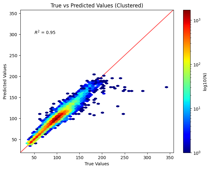
Linear Correlation (Clusters)

from matplotlib import cm

# Calculate R-squared value
r2 = r2_score(y, yhat)

plt.figure(figsize=(8, 6))
plt.hexbin(y, yhat, gridsize=50, cmap=cm.jet, bins='log')
plt.xlabel('True Values')
plt.ylabel('Predicted Values')
plt.title('True vs Predicted Values (Clustered)')

cb = plt.colorbar()
cb.set_label('log10(N)')

# Set the limits of x and y to be the same
lims = [
    np.min([plt.xlim(), plt.ylim()]),  # min of both axes
    np.max([plt.xlim(), plt.ylim()]),  # max of both axes
]

plt.xlim(lims)
plt.ylim(lims)

# Draw the diagonal line
plt.plot(lims, lims, 'r-', alpha=0.75, zorder=0)

# Add R^2 value to the plot
plt.annotate(f'$R^2$ = {r2:.2f}', xy=(50, 300))

plt.show()

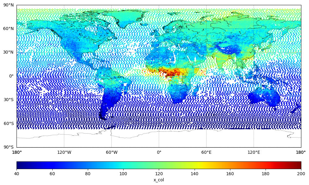
Plot TROPESS XCO (True Value)

latitude = df['lat']
longitude = df['lon']
x_col = y
x_col_hat = yhat

# Specify figure size (in inches)
fig = plt.figure(figsize=(12, 8))  

# Create a basemap instance
m = Basemap(projection='cyl', resolution='l', 
            llcrnrlat=-90, urcrnrlat=90,  # set latitude limits to -90 and 90
            llcrnrlon=-180, urcrnrlon=180)  # set longitude limits to -180 and 180

m.drawcoastlines(linewidth=0.2)
m.drawcountries(linewidth=0.2)

# Draw parallels (latitude lines) and meridians (longitude lines)
parallels = np.arange(-90., 91., 30.)
m.drawparallels(parallels, labels=[True,False,False,False], linewidth=0.3)

meridians = np.arange(-180., 181., 60.)
m.drawmeridians(meridians, labels=[False,False,False,True], linewidth=0.3)    

# Standard catter plot
# Transform lat and lon to map projection coordinates
xlon, ylat = m(longitude, latitude)

# Plot the data using scatter (you may want to choose a different colormap and normalization)
sc = m.scatter(xlon, ylat, c=x_col, cmap='jet', s=10, vmin=40.0, vmax=200.0, marker='.')

# Add a colorbar
cbar = m.colorbar(sc, location='bottom', pad="10%")
cbar.set_label('x_col')

plt.show()

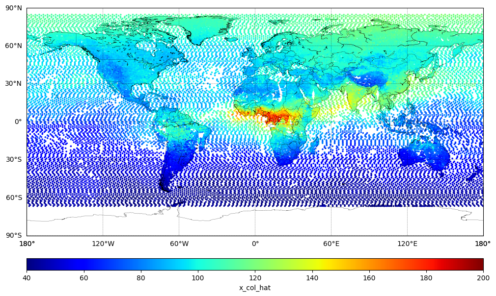
Plot Model XCO (Predicted Value)

# Specify figure size (in inches)
fig = plt.figure(figsize=(12, 8))  

m = Basemap(projection='cyl', resolution='l', 
            llcrnrlat=-90, urcrnrlat=90,  # set latitude limits to -90 and 90
            llcrnrlon=-180, urcrnrlon=180)  # set longitude limits to -180 and 180

m.drawcoastlines(linewidth=0.2)
m.drawcountries(linewidth=0.2)

# Draw parallels (latitude lines) and meridians (longitude lines)
parallels = np.arange(-90., 91., 30.)
m.drawparallels(parallels, labels=[True,False,False,False], linewidth=0.3)

meridians = np.arange(-180., 181., 60.)
m.drawmeridians(meridians, labels=[False,False,False,True], linewidth=0.3)    

# Standard catter plot
# Transform lat and lon to map projection coordinates
xlon, ylat = m(longitude, latitude)

# Plot the data using scatter (you may want to choose a different colormap and normalization)
sc = m.scatter(xlon, ylat, c=x_col_hat, cmap='jet', s=10, vmin=40.0, vmax=200.0, marker='.')

# Add a colorbar
cbar = m.colorbar(sc, location='bottom', pad="10%")
cbar.set_label('x_col_hat')

plt.show()

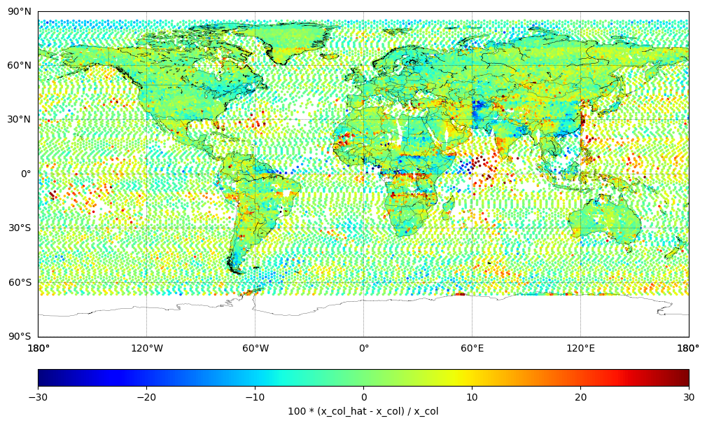
Plot Difference (Predicted - True)

Plot the percentage difference between TROPESS XCO (Truth) and SEARS XCO CrIS ML v1.9 (Predicted):

ydiff = 100 * (x_col_hat - x_col) / x_col
print (f'# of observations: {len(ydiff)}')

# Specify figure size (in inches)
fig = plt.figure(figsize=(12, 8))  

m = Basemap(projection='cyl', resolution='l', 
            llcrnrlat=-90, urcrnrlat=90,  # set latitude limits to -90 and 90
            llcrnrlon=-180, urcrnrlon=180)  # set longitude limits to -180 and 180

m.drawcoastlines(linewidth=0.2)
m.drawcountries(linewidth=0.2)

# Draw parallels (latitude lines) and meridians (longitude lines)
parallels = np.arange(-90., 91., 30.)
m.drawparallels(parallels, labels=[True,False,False,False], linewidth=0.3)

meridians = np.arange(-180., 181., 60.)
m.drawmeridians(meridians, labels=[False,False,False,True], linewidth=0.3)    

# Standard catter plot
# Transform lat and lon to map projection coordinates
xlon, ylat = m(longitude, latitude)

# Plot the data using scatter (you may want to choose a different colormap and normalization)
sc = m.scatter(xlon, ylat, c=ydiff, cmap='jet', s=10, vmin=-30.0, vmax=+30.0, marker='.')

# Add a colorbar
cbar = m.colorbar(sc, location='bottom', pad="10%")
cbar.set_label('100 * (x_col_hat - x_col) / x_col')

plt.show()

# of observations: 40470

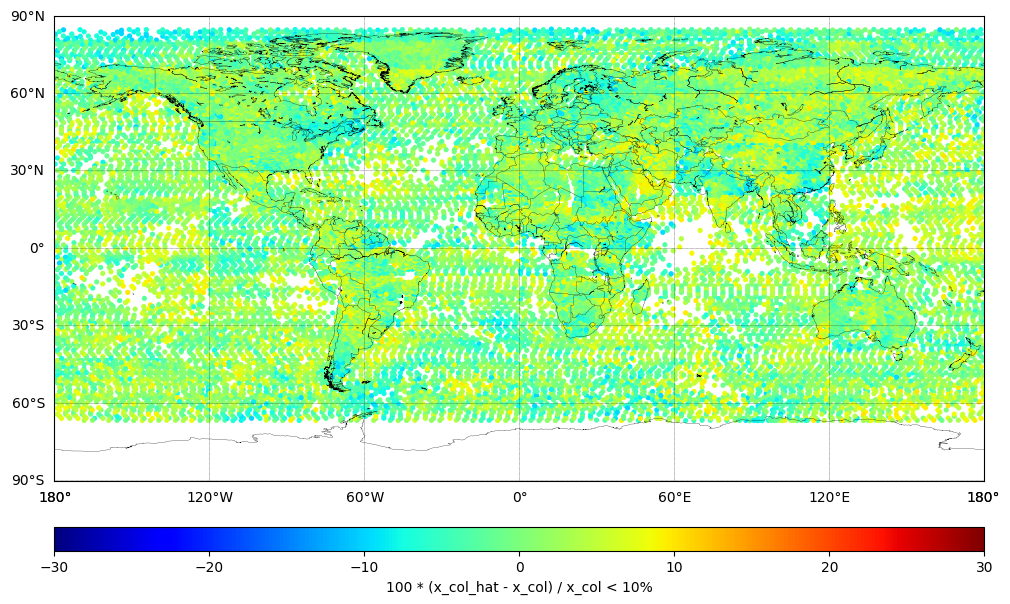
Plot Difference (less than 10%)

Plot the percentage difference between the TROPESS XCO (Truth) and the SEARS XCO CrIS ML v1.9 (Predicted) where the difference is less than 10%:

ydiff = 100 * (x_col_hat - x_col) / x_col
print (f'# of observations: {len(ydiff)}')

ydiff_10_index = np.where(abs(ydiff) < 10)[0]
ydiff_10 = ydiff[ydiff_10_index]
print (f'# of observations where difference < 10%: {len(ydiff_10)}')

latitude_10 = latitude[ydiff_10_index]
longitude_10 = longitude[ydiff_10_index]

# Specify figure size (in inches)
fig = plt.figure(figsize=(12, 8))  

m = Basemap(projection='cyl', resolution='l', 
            llcrnrlat=-90, urcrnrlat=90,  # set latitude limits to -90 and 90
            llcrnrlon=-180, urcrnrlon=180)  # set longitude limits to -180 and 180

m.drawcoastlines(linewidth=0.2)
m.drawcountries(linewidth=0.2)

# Draw parallels (latitude lines) and meridians (longitude lines)
parallels = np.arange(-90., 91., 30.)
m.drawparallels(parallels, labels=[True,False,False,False], linewidth=0.3)

meridians = np.arange(-180., 181., 60.)
m.drawmeridians(meridians, labels=[False,False,False,True], linewidth=0.3)    

# Standard catter plot
# Transform lat and lon to map projection coordinates
xlon, ylat = m(longitude_10, latitude_10)

# Plot the data using scatter (you may want to choose a different colormap and normalization)
sc = m.scatter(xlon, ylat, c=ydiff_10, cmap='jet', s=30, vmin=-30.0, vmax=+30.0, marker='.')

# Add a colorbar
cbar = m.colorbar(sc, location='bottom', pad="10%")
cbar.set_label('100 * (x_col_hat - x_col) / x_col < 10%')

plt.show()

# of observations: 40470
# of observations where difference < 10%: 37666